Estimating the effectiveness of DCP - Part 1
[This is the first of two posts I wrote on estimating the cost-effectiveness of the DCP organization, who themselves publish excellent reports on the cost-effectiveness of health interventions. It was originally published on the Giving What We Can blog.]
When searching for high-effectiveness charities, there are a few resources that incredibly useful. One of those is the reports of the Disease Control Priorities Project, which provide an analysis of the cost-effectiveness of a great number of health interventions.
Given the value of this data, we might wonder just how valuable this information is, and whether it might be worth donating to DCP to produce more of it.
In this post I will present a statistical model (designed by myself and Nick Dunkley) for estimating the effectiveness of donating to DCP. Although this is going to over-simplify the situation, it should be able to give us a ballpark estimate.
Here’s the idea. Firstly, we assume that DCP has some number of followers who make their donation decisions based on DCP’s recommendations; that is, they put their donations towards whatever intervention DCP recommends most highly. If DCP says the best thing is buying hang-gliders for kittens, then that’s where they’ll send their money. So the current situation would have all that money going towards the intervention that the DCP2 report claims is most effective. We’ll refer to the money donated as DCP’s “money moved”. Furthermore, we’ll assume that this money is all translated into DALYs at the rate that DCP claims.
Now, suppose that there’s a big bag of interventions that DCP assesses. Then we assume that for some amount of money, DCP can pick a random intervention from the bag and accurately assess its effectiveness. If it comes out better their current best recommendation, then when they report this fact, all of their followers will shift their donations to the new best intervention.
If this is a good model of how DCP works, then we now have enough information to work out how much good we can do by donating to DCP. I’m going to be using R, a statistics package, to do the heavy lifting - it’s free and I’ve attached the script I used if you’re keen and want to check my working!
Firstly, we need to know something about the distribution of the interventions in the bag. A quick reminder about probability distributions: the probability distribution of some random variable usually looks like a humped graph. Along the bottom are all the options we could have. In this case, that’s the possible cost-effectivenesses of a random health intervention, i.e. pretty much any positive real number. Along the side it shows how likely that possibility is. One very common type of distribution is a “normal” distribution. This just looks like a big hump in the middle that spreads out to the sides (often called a “bell-curve”). Intuitively, that means that most of the time you get one of the possibilities in the middle, and the other possibilities get less likely as they get further away from the middle. Normal distributions are quite nice to work with, and they’re also pretty common. Importantly, they can be totally specified by just two parameters: the mean of the distribution (the average outcome you get), and the standard deviation (which tells you how far away from the mean things tend to be). Between the two of these you know where the middle of the hump is (the mean), and how wide it is (the standard deviation), and that’s all you need to know.
Back to our health interventions. Fortunately, we have a lot of data from DCP about the cost-effectiveness of interventions: if we plot the effectiveness of the interventions they assessed in the DCP2 report, we get a distribution that looks a bit like this:
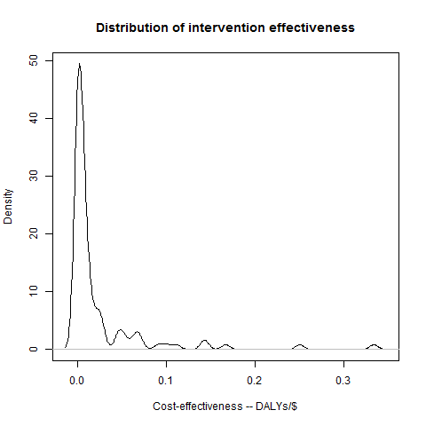
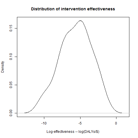
That’s definitely not a normal distribution, but it is a “log-normal” distribution. A log-normal distribution is fairly straightforward: if you take the logarithms of all the possibilities along the bottom, and then plot the distribution, you should get a normal distribution. And if we do that for the DCP data, then we do indeed get a very plausible-looking bell-curve.
Now, this makes it looks pretty plausible that the DCP data really does follow a (log-)normal distribution, and it’ll be helpful if we can work out the two parameters for it that I mentioned above. For the moment, let’s assume that taking the mean and standard deviation of the logarithms of the data gives us the right parameters - we can be more sophisticated (in particular we’re going to want to think about the possibility of error), but I’ll leave that for a later post.
Having the parameters for the distribution means that we can get R to make up entirely new data points as if they came from the original data set. And if the actual data really is distributed in the way we think it is, then this is a lot like DCP finding and assessing a new random intervention. We can then do the rest of our model process - check whether it’s a better charity than we had before, and if so work out what the difference is - and get an answer for how much difference that one attempt would make. We can then use R to simulate doing this a large number of times, and then simply average the results! Thus: we generate a large number of samples, to represent a large number of investigations by DCP. We can then work out the difference in effectiveness between each “new” intervention and the current best option. The current best option is better than average, so we’ll expect the difference in general to be negative. We can regard all those results as 0, however, as in that case there would (in our model) be no change in where the money goes.
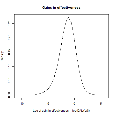
(Looking at the graph we get, the improvements also appear to be also log-normally distributed). Finally, we can then average these results. Call that average A.
At this point, we need to plug in two final, very important parameters. These are figures for the money moved (M), and for the cost of DCP doing an investigation (C). These are particularly important as the our final estimate is going to be the average good done by an investigation (A*M), divided by the cost of doing it (C). Our final estimate will therefore be directly proportional to M, and inversely proportional to C. We’ll discuss these a little more in a future post. For now, I’m just going to give you some figures that are at least the right order of magnitude: namely about \$530 million for M, and about \$200,000 for C.
Putting all this together, we get an estimate for the effectiveness of DCP of a staggering 89 DALYs/\$! For comparison, the best intervention that DCP claims to have found so far clocks in at 0.33 DALYs/\$! As mentioned earlier, of course, this estimate is only as good as our model, but it certainly looks promising. In the next post I’ll talk about how we can improve the model in a couple of ways.
A few final caveats:
- This kind of research will be a high-variance strategy: most of the time nothing useful will happen, but occasionally there will be really, really good outcomes.
- The hidden parameter in this model is the effectiveness of DCP’s current strongest recommendation. In particular, if new interventions are discovered that have much higher effectiveness, then the need to do further research drops.
- These results are not immediately applicable to charity-evaluators such as GiveWell. GiveWell looks at charities, not interventions, and we don’t have a data-set for that in the way that we have for DCP. It may be that if we make some assumptions we might be able to adapt the data, but this is an open question.